Question 1 (a)
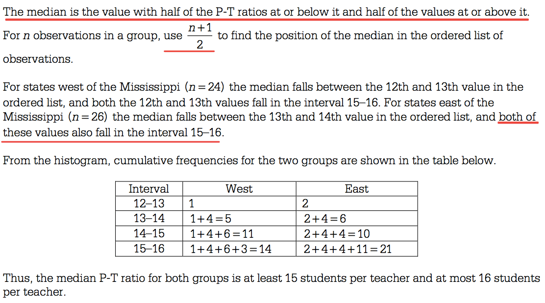
Estimation for median
Question 1 (c)
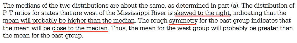
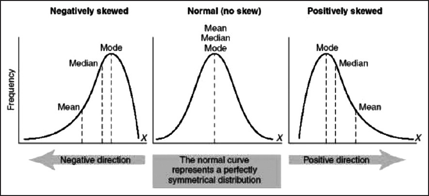
Mean, Median, and Skew
Question 1 (a)

Question 3 (a)
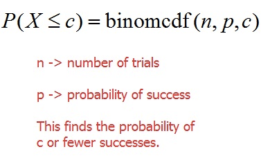
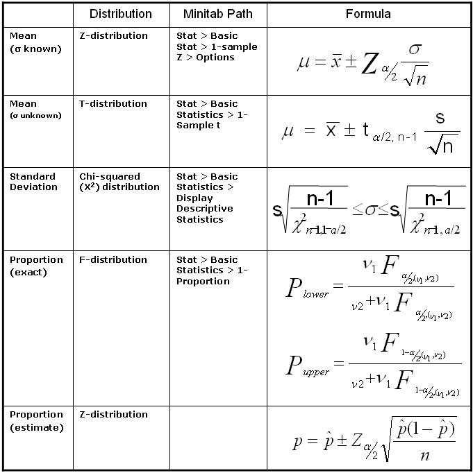
Pay attention to the notation
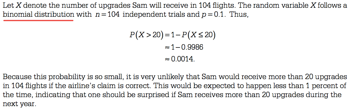
Question 3 (b)
Binomial distribution
Question 3 (c)
Question 4 (b)
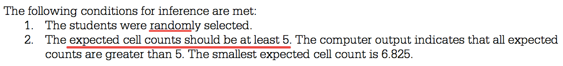
Conditions for a chi-square inference procedure
Question 4 (d)
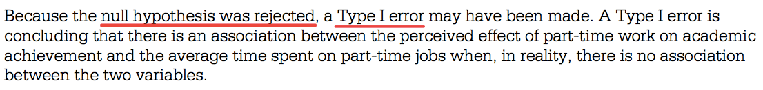
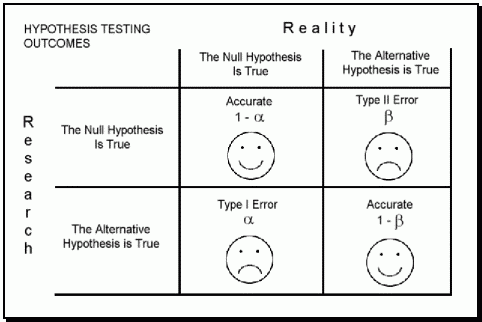
Type I error and Type II error
Question 5 (a)
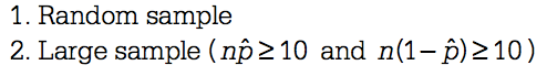
Conditions for one-proportion Z interval
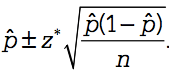
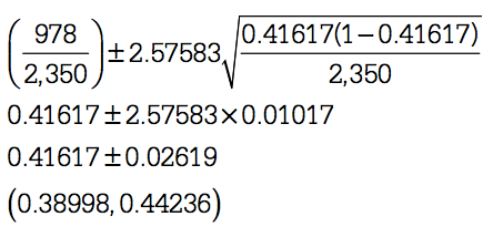
Calculation for one-proportion Z interval
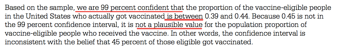
Interpretation for one-proportion Z interval
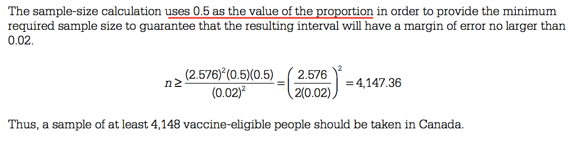
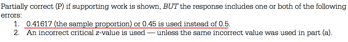
Question 5 (b)
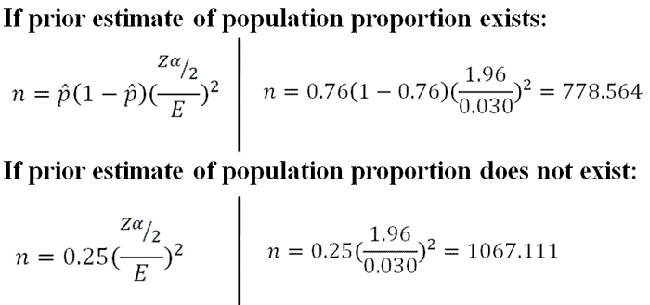
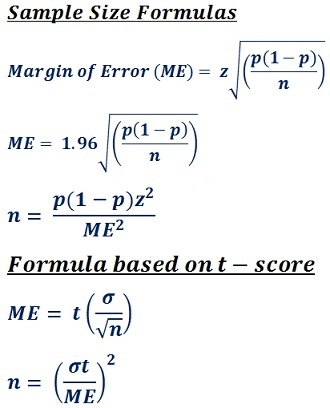
Calculating Required Sample Size to Estimate Population Mean
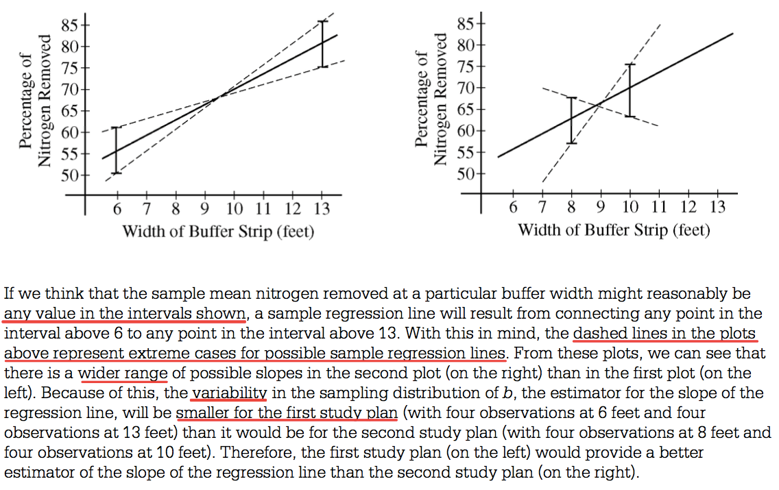
Question 6 (b)

Question 6 (c)
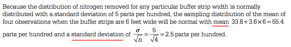
Describe distribution: Mean & Standard deviation
Question 6 (d)
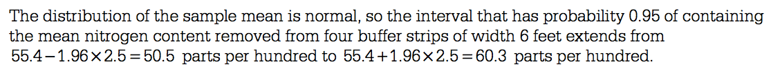
Confidence interval
Question 6 (e)
Question 6 (f)